Comparing Clustering Methods on the Same Dataset

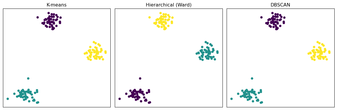
K-means, hierarchical clustering, and DBSCAN applied to the same simulated ecological dataset — and why they disagree.

The analytical question

Given a set of samples described by several continuous environmental variables (e.g. temperature, oxygen, salinity), do they form distinct groups — and does the answer depend on which clustering method you use?

Data source

This post uses a simulated dataset of 150 samples with three underlying groups, generated with scikit-learn’s make_blobs, plus one method (DBSCAN) evaluated on a non-globular shape to show where k-means style methods fail. No real project or confidential data is used.

Data cleaning

Simulated data is already clean; in practice this step would include checking for missing values, standardizing variable scales (important here — clustering is scale-sensitive), and screening for outliers.

Statistical method

Three methods are compared on the same standardized data: k-means (assumes roughly spherical, similarly-sized clusters), agglomerative hierarchical clustering (Ward linkage), and DBSCAN (density-based, no assumption of cluster shape).

Code

import numpy as np
from sklearn.datasets import make_blobs
from sklearn.preprocessing import StandardScaler
from sklearn.cluster import KMeans, AgglomerativeClustering, DBSCAN
import matplotlib.pyplot as plt

rng = np.random.default_rng(42)
X, y_true = make_blobs(n_samples=150, centers=3, cluster_std=0.9, random_state=42)
X = StandardScaler().fit_transform(X)

kmeans = KMeans(n_clusters=3, n_init=10, random_state=42).fit_predict(X)
hier = AgglomerativeClustering(n_clusters=3, linkage="ward").fit_predict(X)
dbscan = DBSCAN(eps=0.4, min_samples=5).fit_predict(X)

fig, axes = plt.subplots(1, 3, figsize=(12, 4))
for ax, labels, name in zip(
    axes, [kmeans, hier, dbscan], ["K-means", "Hierarchical (Ward)", "DBSCAN"]
):
    ax.scatter(X[:, 0], X[:, 1], c=labels, cmap="viridis", s=25)
    ax.set_title(name)
    ax.set_xticks([]); ax.set_yticks([])
plt.tight_layout()
plt.show()

Visualization

The figure above shows the same simulated samples colored by cluster assignment under each method.

Interpretation

On this well-separated, roughly spherical simulated dataset, all three methods agree closely with the true grouping. That agreement is the exception, not the rule: as soon as clusters vary in density, size, or shape, k-means and Ward-linkage hierarchical clustering (which both implicitly assume compact, similarly-sized groups) start to disagree with density-based methods like DBSCAN — and neither is “more correct” without external validation.

Assumptions

• K-means and Ward-linkage clustering assume clusters are roughly convex/spherical and similar in size.
• DBSCAN assumes clusters are contiguous regions of similar density and requires tuning eps/min_samples, which is data-scale-dependent.
• All three assume standardized (comparable-scale) input features; skipping standardization here would let higher-variance variables dominate the distance calculations.

Limitations

Cluster number was fixed at k=3 for k-means/hierarchical for illustration; in practice this should be chosen via a validation criterion (e.g. silhouette score, gap statistic) rather than assumed. Real ecological or microbiome data rarely produces clusters this well-separated — treat this as a demonstration of method behavior, not a recommendation to trust any single method’s output at face value.

Reproducibility

scikit-learn, numpy, matplotlib — see environment.yml in the tutorial repository (placeholder — link to your actual environment file when publishing). Random seed fixed (random_state=42) for exact reproducibility of this simulated example.